4 min read
CRM software for high-performance sales teams
When first introduced to forecasting field sales managers usually come across two differentiating types: quantitative methods of sales forecasting and qualitative methods of sales forecasting. Before we get started let’s get a quick definition of the two:
Quantitative Methods of Sales Forecasting
Based on mathematical (quantitative) models, they use objective sets of historical sales data to predict likely revenue increases in the future.
Qualitative Methods of Sales Forecasting
Based on subjective feedback, emotions or opinions from people normally within the related industry. These would typically include market research reports, expert focus groups and the Delphi method, most applicable when entering a new market where little data is readily available.
And, as the title suggests, it’s the quantitative methods of sales forecasting that we are going to be focusing on this article. They tend to be slightly more accurate as you are using real data in order to make your predictions. However, no sales forecasting technique is perfect and I seriously doubt your sales reports will be predicting right down to the penny what the next month’s revenue increases will be.
Now although the word “quantitative” comes saddled with a lot of mathematical connotations (and it does indeed include a little bit of numbery work on your part) it’s nothing to get too worked up about.
I’m horrible at math, yet manage these methods just fine.
Keeping it simple is the name of the game and the four methods I’m going to introduce you to now are some of the most commonly used across the industry. Known as the time-series models, they attempt to predict future sales by applying patterns found in historical data sets.
The first one we are going to look at is known simply as the historical growth rate.
Essentially what you’re doing here is using the data from a set period of time, this could be anything from weeks, to months or even years, depending on the type of forecast you are looking to draw up to predict the next period’s growth rate.
So for example, let’s suppose you are trying to predict next month’s sales.
You would multiply this month’s sales by one, plus the monthly sales growth rate.
The formula would therefore look like this:
(x) month’s sales x (1 + % rate of sales growth) = next month’s sales
So if you had a 20% increase in sales over the past month, and you sold say, $25,000 worth of product, then your sales forecast for next month would be:
$25,000 x (1 + 20%) = $30,000
Simple!
Another set of quantitative methods of sales forecasting we are going to look at are linear extensions. To put it simply, linear extensions work by plotting your historic sales data on a chart, drawing a line through the middle of the points and extending this line in to the future.
Let us plot some sales data into a standard line chart in Excel.
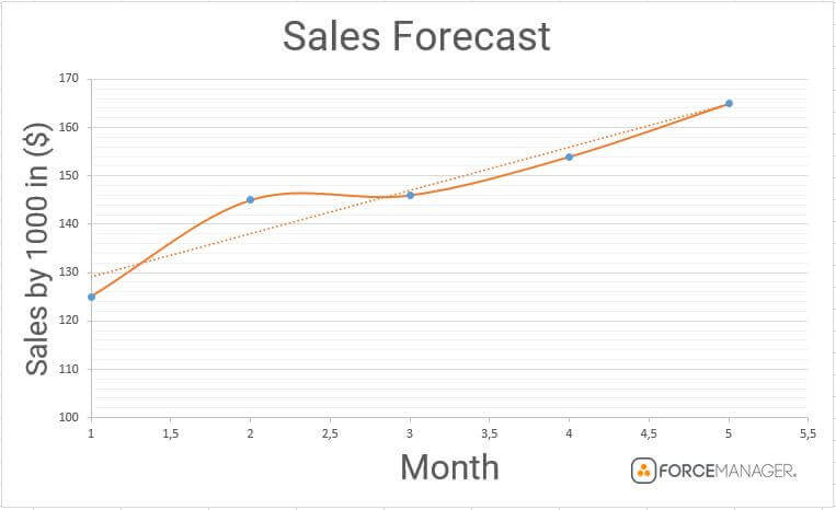
The (y) vertical axis are sales, represented by increments of $10K and the (x) horizontal axis refers to a period of time, in this case represented by month.
In order to forecast sales for the upcoming month you can use the TREND feature found in excel (I’ll leave a tutorial right here) or alternatively you can click on the data line shown on the graph, and as you do so a pop up will appear to the right of the excel sheet. Click the “bar graph” icon and a drop down list will appear with options to extend a tendency line past your input data (x).
You will end up with something similar to this:
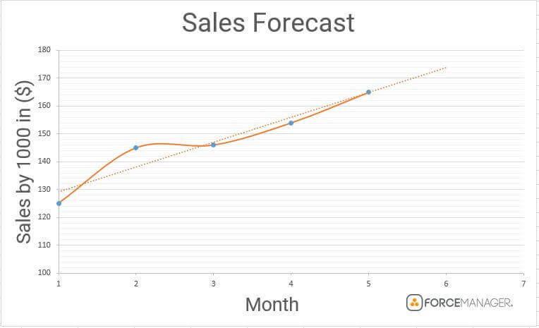
Where this line intersects your forecast date will be your predicted forecast revenue. In this case the line intercepts (x) month 6 at (y) 172.
Therefore our sales forecast for month 6 using the linear method is: $172,000
However, the linear extension does have its drawbacks. As most sales managers will attest to sales revenue rarely increases in a linear fashion i.e. what you made in April will be increased by (x) amount in May because we saw the same trend happen between March – April.
That’s because it can’t account for seasonality. If you sell mulled wine for example I’d expect to see a spike in sales as the temperature winds down and we head into the Winter period. Therefore using extrapolated data from the mulled wine sold between the months of May – September is not going to accurately reflect this expected spike in sales (unless of course there are lot of you who enjoy mulled wine in summer!).
The run rate is an average calculated from past historical sales data and is represented by:
total revenue / sum of past sales periods
So let’s imagine we are in April and your sales periods are broken into months, and as of this moment you’ve sold $32,000 worth of product.
That means your monthly revenue averages out at $8000.
Now in order to predict your overall revenue for the year you will need to calculate the expected amount sold over the remaining 8 months.
So if your average is $8000 a month:
8 x $8000 = $64,000
For a grand sum annual total of:
$64,000 + $32,000 = $96,000
As you can see the run rate method works best when trying to forecast revenue for the remainder of a set period of time. For example, if investors have given you (x) target to hit by (y) months time before they release more equity into the business, you could employ the run rate technique to quickly gauge whether that’s likely to happen or not.
One of the final sets of quantitative methods of sales forecasting we are going to look at is the Simple Moving Average. Similar to run rate, it requires you extrapolate sales data from a set period only this time that period is dynamic – it moves forward depending on the timeframe we are looking at.
Let me give you an example:
Say you want to predict sales for the next 6 months. You have sales data from the past 3 years from which to extrapolate your forecast which gives exactly 6x (6) month periods to work with.
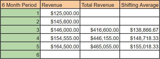
As you can see from the graph the simple moving average for 6 month periods 1-3 is: $138,866.67
This was calculated by adding the revenue from the first three 6 month periods: $125,000 + $145,600 + 146,000 = $416,600 and then dividing by three (to give you the average) = $138,866.67
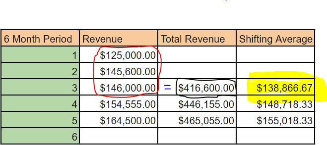
Now this where we differentiate from run rate.
Because this is a simple moving average, everything moves forward by 1, 6 month period.
So we will repeat the same process for periods 2-4:
And again for periods 3-5:
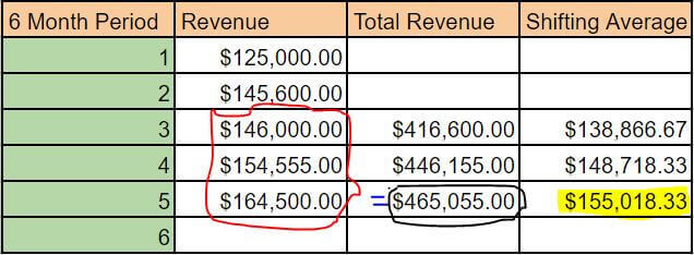
So when trying to forecast the revenue for 6th period, you simply use the shifting average from period 5:
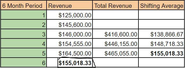
Out of the other quantitative methods of sales forecasting we’ve looked at shifting average tends to be slightly more accurate as it takes a dynamic average. As you can see total revenue is steadily increasing over each 6 month period. If we solely used the run rate from periods 1-3 it wouldn’t account for the steady increase in revenue from periods 3-5, leaving your forecast period 6 woefully short of it’s likely revenue.
In conclusion you can see that all quantitative methods of sales forecasting have their positives and negatives. To find out which one best suits your sales process it will take a bit of preparation on your part. Essentially, if your industry is pretty stable without too much annual fluctuation then most of these methods will be applicable, but if you work in fashion, retail or tourism you can expect a lot of fluctuation from seasonality, so picking a moving forecast maybe a better option. So make sure to do your research before getting stuck in!